2. Sinusoidal wave in a headland channel
2.1. Introduction
This example simulates the flow in a headland channel with oscillating head-driven flow. It shows how to
read in an external mesh file;
apply boundary conditions for a sinusoidal, head-driven flow;
solve the transient shallow water equations;
compute vorticity of the flow field;
save output files to disk.
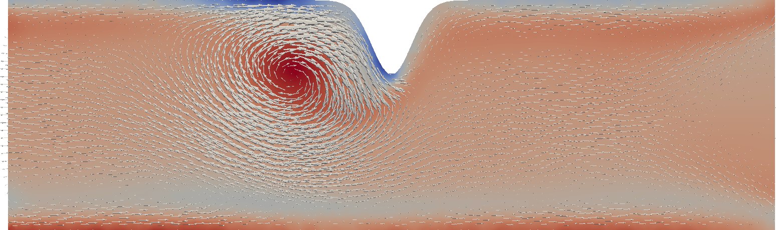
The following plot shows the vorticity function with velocity glyphs after a few timesteps:
The equations to be solved are the shallow water equations
where
\(u\) is the velocity,
\(\eta\) is the free-surface displacement,
\(H=\eta + h\) is the total water depth where \(h\) is the water depth at rest,
\(c_b\) is the (quadratic) natural bottom friction coefficient,
\(\nu\) is the viscosity coefficient,
\(g\) is the gravitational constant.
2.2. Implementation
We begin with importing the OpenTidalFarm module.
from opentidalfarm import *
Next we get the default parameters of a shallow water problem and configure it to our needs.
prob_params = SWProblem.default_parameters()
First we define the computational domain. We load a previously generated mesh
(using `Gmsh` and converted with `dolfin-convert`):
domain = FileDomain("mesh/headland.xml")
prob_params.domain = domain
Next we specify the boundary conditions. The parameter t in the
dolfin.Expression is special in OpenTidalFarm as it will be
automatically updated to the current timelevel during the solve.
# We assume a propagating wave in the headland case and compute the phase
# difference to drive flow in the channel.
tidal_amplitude = 5.
tidal_period = 12.42*60*60 # M2 tidal period
H = 40 # channel depth
eta_channel = "amp*sin(omega*t + omega/pow(g*H, 0.5)*x[0])"

bcs = BoundaryConditionSet()
eta_expr = Expression(eta_channel, t=Constant(0), amp=tidal_amplitude,
                      omega=2*pi/tidal_period, g=9.81, H=H)
bcs.add_bc("eta", eta_expr, facet_id=1, bctype="strong_dirichlet") # west
bcs.add_bc("eta", eta_expr, facet_id=2, bctype="strong_dirichlet") # east
bcs.add_bc("u", Constant((0, 0)), facet_id=3, bctype="strong_dirichlet")  # coast

prob_params.bcs = bcs
The other parameters are straight forward:
# Equation settings
prob_params.viscosity = Constant(40)
prob_params.depth = Constant(H)
prob_params.friction = Constant(0.0025)
# Temporal settings
prob_params.theta = Constant(0.6)
prob_params.start_time = Constant(0)
prob_params.finish_time = Constant(tidal_period*5)
prob_params.dt = Constant(tidal_period/100)
# The initial condition consists of three components: u_x, u_y and eta
# Note that we do not set all components to zero, as some components of the
# Jacobian of the quadratic friction term is non-differentiable.
prob_params.initial_condition = Expression(("DOLFIN_EPS", "0", eta_channel), t=Constant(0),
              amp=tidal_amplitude, omega=2*pi/tidal_period, g=9.81, H=H)
Here we only set the necessary options. A full option list with its current values can be viewed with:
print prob_params
Once the parameter have been set, we create the shallow water problem:
problem = SWProblem(prob_params)
Next we create a shallow water solver. Here we choose to solve the shallow water equations in its fully coupled form. Again, we first ask for the default parameters, adjust them to our needs and then create the solver object.
sol_params = CoupledSWSolver.default_parameters()
sol_params.dump_period = -1
solver = CoupledSWSolver(problem, sol_params)
In this example we would also like to compute the vorticity of the flow field. The following FEniCS code solves for the vorticity by a L2 projection
class VorticitySolver(object):
    def __init__(self, V):
        self.V = V
        self.u = Function(V)
        Q = V.extract_sub_space([0]).collapse()

        r = TrialFunction(Q)
        s = TestFunction(Q)
        a = r*s*dx
        self.L = (self.u[0].dx(1) - self.u[1].dx(0))*s*dx
        self.a_mat = assemble(a)

        self.vort = Function(Q)

    def solve(self, u):
        self.u.assign(project(u, V))
        L_mat = assemble(self.L)
        solve(self.a_mat, self.vort.vector(), L_mat, annotate=False)
        return self.vort
We also create some output files to store the results
u_xdmf = XDMFFile("outputs/u.xdmf")
eta_xdmf = XDMFFile("outputs/eta.xdmf")
vort_xdmf = XDMFFile("outputs/vorticity.xdmf")
u_xdmf.parameters["flush_output"] = True
eta_xdmf.parameters["flush_output"] = True
vort_xdmf.parameters["flush_output"] = True
Extract the velocity function space and initialised the vorticity solver
V = solver.function_space.extract_sub_space([0]).collapse()
vort_solver = VorticitySolver(V)
Now we start the time loop
for s in solver.solve(annotate=False):
    print "Computed solution at time %f" % s["time"]

    # Write velocity, surface elevation and vorticity to files
    u_xdmf.write(s["u"], s["time"])
    eta_xdmf.write(s["eta"], s["time"])

    vort = vort_solver.solve(s["u"])
    vort_xdmf.write(vort, s["time"])
The results are stored in the outputs directory and can be viewed with [Paraview](http://www.paraview.org/).
The inner part of the loop is executed for each timestep. The variable s
is a dictionary and contains information like the current timelevel, the velocity and
free-surface functions.
2.3. How to run the example
The example code can be found in examples/headland-simulation/ in the
OpenTidalFarm source tree, and run with:
$ python headland-simulation.py