7. Sensitivity analysis
7.1. Introduction
Gradient information may also be used to analyse the sensitivity of the chosen functional to various model parameters - for example the bottom friction:
This enables the designer to identify which parameters may have a high impact upon the quality of the chosen design (as judged by the choice of functional).
- This example shows how to:
set up shallow water solver with a turbine farm;
define an objective, here the farms power production;
- compute the sensitivity of this objective with respect to:
viscosity;
depth;
bottom friction.
7.2. Implementation
As with other examples, we begin by defining a steady state shallow water problem, once more this is similar to the Sinusoidal wave in a channel example except that we define steady flow driven by a 0.1 m head difference across the domain. Note that this is facilitated by defining a strong dirichlet boundary condiditon on the walls:
from opentidalfarm import *

# Create a rectangular domain.
domain = FileDomain("mesh/mesh.xml")

# Specify boundary conditions.
bcs = BoundaryConditionSet()
bcs.add_bc("eta", Constant(0.1), facet_id=1)
bcs.add_bc("eta", Constant(0), facet_id=2)
# The no-slip boundary conditions.
bcs.add_bc("u", Constant((0, 0)), facet_id=3, bctype="strong_dirichlet")
Set the shallow water parameters, since we want to extract the spatial variation of the sensitivity of our model parameters, rather than simply defining constant values, we define fields over the domain (in this case we’re simply defining a field of a constant value, using dolfin’s interpolate.
prob_params = SteadySWProblem.default_parameters()
prob_params.domain = domain
prob_params.bcs = bcs
V = FunctionSpace(domain.mesh, "CG", 1)
prob_params.viscosity = interpolate(Constant(3), V)
prob_params.depth = interpolate(Constant(50), V)
prob_params.friction = interpolate(Constant(0.0025), V)
The next step is to specify the array design for which we wish to analyse the sensitivity. For simplicity we will use the starting guess from the Farm layout optimization example; 32 turbines in a regular grid layout. As before we’ll use the default turbine type and define the diameter and friction. In practice, one is likely to want to analyse the sensitivity of the optimised array layout - so one would substitute this grid layout with the optimised one.
turbine = BumpTurbine(diameter=20.0, friction=12.0)
farm = RectangularFarm(domain, site_x_start=160, site_x_end=480,
                       site_y_start=80, site_y_end=240, turbine=turbine)
farm.add_regular_turbine_layout(num_x=8, num_y=4)
prob_params.tidal_farm = farm
Now we can create the shallow water problem
problem = SteadySWProblem(prob_params)
Next we create a shallow water solver. Here we choose to solve the shallow water equations in its fully coupled form:
sol_params = CoupledSWSolver.default_parameters()
sol_params.dump_period = -1
solver = CoupledSWSolver(problem, sol_params)
We wish to study the effect that various model parameters have on the
power. Thus, we select the PowerFunctional
functional = PowerFunctional(problem)
First let’s compute the sensitivity of the power with respect to the turbine
positions. So we set the “control” variable to the turbine positions by using
TurbineFarmControl. We then intialise the ReducedFunctional
control = TurbineFarmControl(farm)
rf_params = ReducedFunctional.default_parameters()
rf = ReducedFunctional(functional, control, solver, rf_params)
m0 = rf.solver.problem.parameters.tidal_farm.control_array
j = rf.evaluate(m0)
turbine_location_sensitivity = rf.derivative(m0)

print "j for turbine positions: ", j
print "dj w.r.t. turbine positions: ", turbine_location_sensitivity
Next we compute the sensitivity of the power with respect to bottom friction.
We redefine the control variable using the class Control into which
we pass the parameter of interest
control = Control(prob_params.friction)
Turbine positions are stored in different data structures (numpy arrays)
than functions such as bottom friction (dolfin functions), so we need to
use a different reduced functional; the FenicsReducedFunctional
rf = FenicsReducedFunctional(functional, control, solver)
j = rf.evaluate()
dj = rf.derivative(project=True)[0]
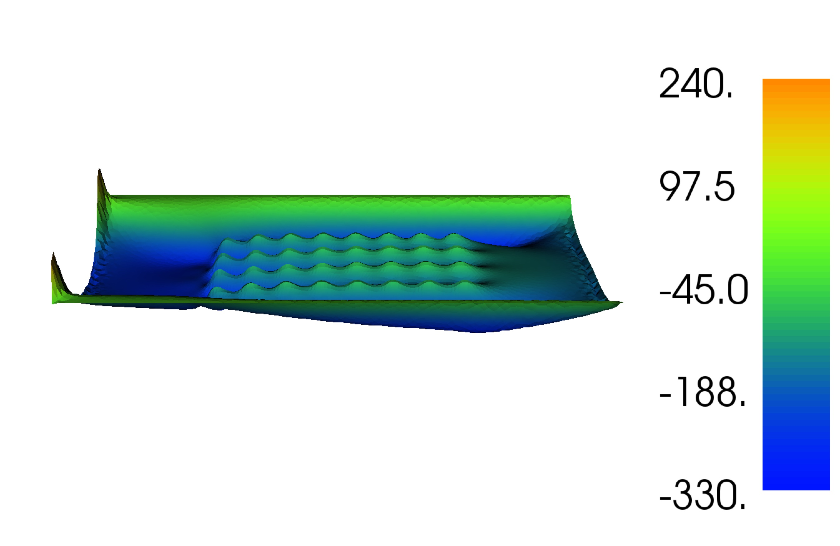
plot(dj, interactive=True, title="Sensitivity with respect to friction")
file = File("FrictionSensitivity.pvd")
file << dj
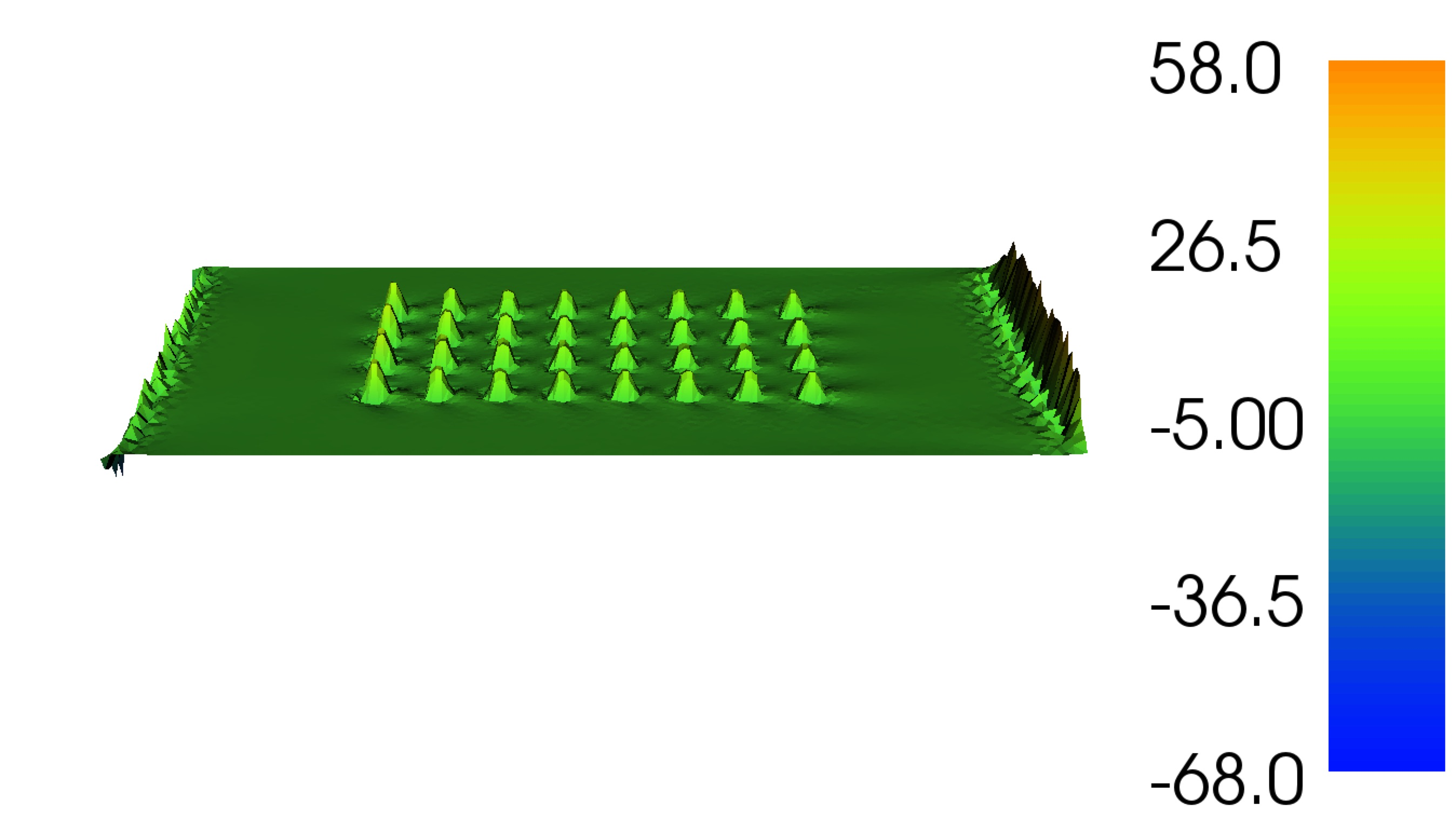
Now compute the sensitivity with respect to depth
control = Control(prob_params.depth)
rf = FenicsReducedFunctional(functional, control, solver)
j = rf.evaluate()
dj = rf.derivative(project=True)[0]
print "j with depth = 50 m: ", j
plot(dj, interactive=True, title="Sensitivity with respect to depth at 50m")
file = File("50mDepthSensitivity.pvd")
file << dj
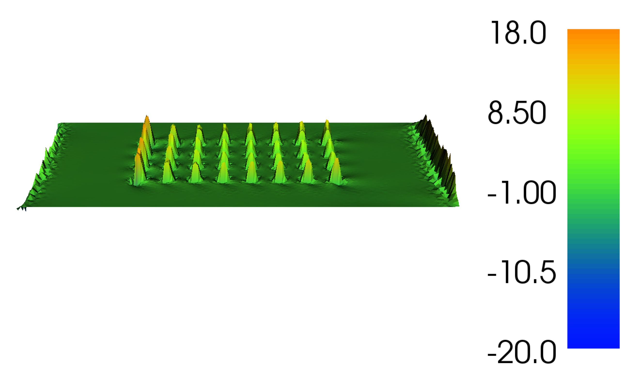
Let’s reduce the depth and reevaluate derivative
prob_params.depth.assign(Constant(10))
j = rf.evaluate()
dj = rf.derivative(project=True)[0]
print "j with depth = 10 m: ", j
plot(dj, interactive=True, title="Sensitivity with respect to depth at 10m")
file = File("10mDepthSensitivity.pvd")
file << dj
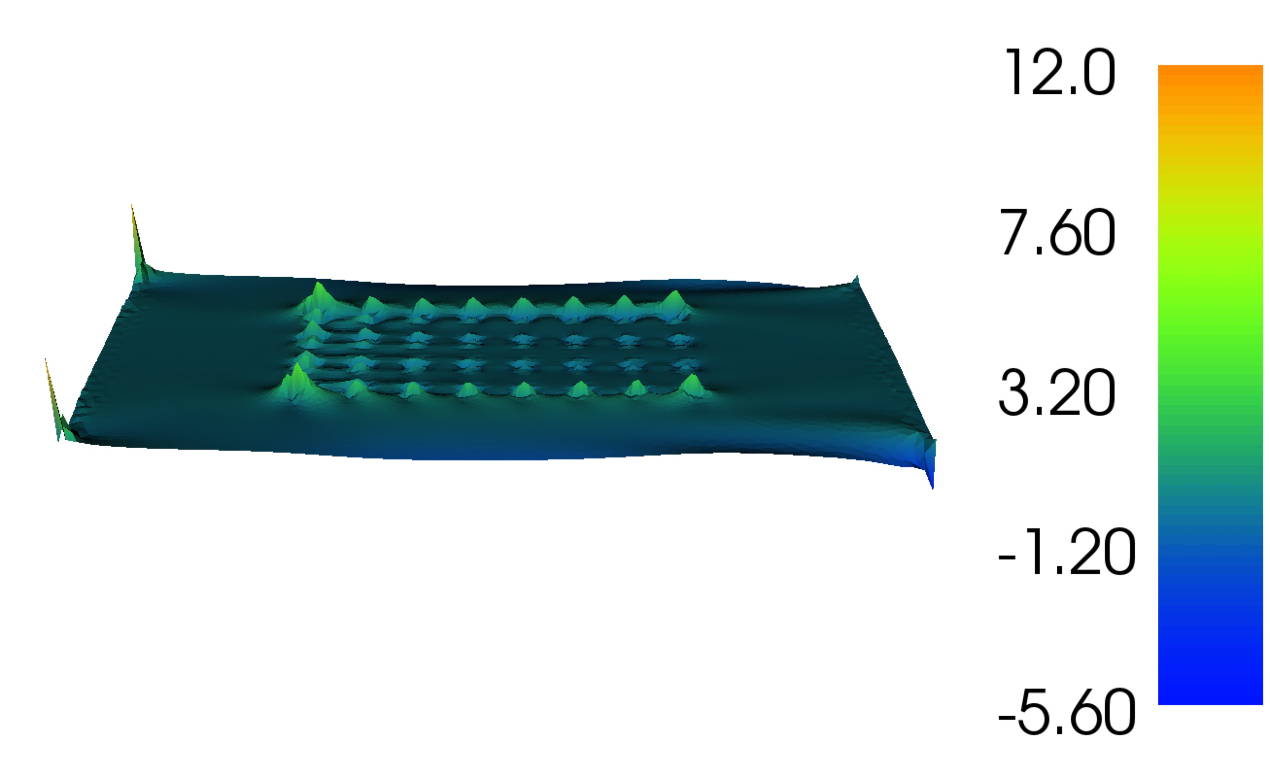
Finally let’s compute the sensitivity with respect to viscosity
control = Control(prob_params.viscosity)
rf = FenicsReducedFunctional(functional, control, solver)
j = rf.evaluate()
dj = rf.derivative(project=True)[0]
plot(dj, title="Sensitivity with respect to viscosity")
file = File("ViscositySensitivity.pvd")
file << dj

interactive() # (For docker users the plots will not be shown, but they are
              #  stored in pvd-files. These files can view with ParaView.)
7.3. How to run the example
The example code can be found in examples/channel-sensitivity/ in the
OpenTidalFarm source tree, and executed as follows:
$ python channel-sensitivity.py